Normally, when we think of MS Access, we do so in the context of database development; that is to say, as software to create database applications for long term use to keep track of data such as customer orders, income and expenditure, and stock control. Such database applications are used by one or more people over a period of time to store, process and retrieve information, and often support the day to day operation of a business.
In this tutorial, however, we are going to look at how MS Access can be used in the context of data analysis. This use is very much different from the database development model described above. Rather than setting up a database for long term use in the day to running of a business operation for example, we are going to use Access in a short term context, as a tool to import data from an external source, and then analyse that data through Access Queries to make it meaningful from a particular perspective. This summarised data can be presented to, say, a management team to make informed decisions based on what the information reveals.
To do this we are going to be working with 2023 house sale data for the Salford area of Greater Manchester. The process will involve extracting a dataset from the UK based HM Land Registry website, importing the dataset into Access, creating query's to categorise and aggregate the data, and then create a report containing a clustered column chart to present the data visually.
Downloading the Dataset
The first step in the process is to download the dataset from the
HM Land Registry website. This will involve filling in an online webform to specify the data we require. In our case this is
all data between
1st January and 31st December 2023 in the district of
SALFORD.
1. Click this link the
HM Land Registry link to open the web form in your browser.
2. Enter "SALFORD" in the DISTRICT textbox, 01/01/2023 and 31/12/2023 for the DATE range (note the UK date format) , and select "ALL" from the HOW MANY RESULTS option group at the bottom.
3. Click the SHOW RESULTS button.
This opens a new web page showing 2947 property sale transactions for 2915 properties. We now need to download the results into a CSV file.
4. Click the DOWLOAD DATA button at the top of the form. This opens a web page giving us options for downloading:
5. Click GET ALL RESULTS AS CSV WITH HEADERS button to start the download.
A dataset called ppd_data.csv will be saved to your downloads folder. You can now open the file to inspect the data. It will open in MS Excel by default and if you scroll to the bottom of the worksheet there should be 2947 rows.
Importing the Dataset into Access
We can now go ahead and import the data into our Access Database.
1. Click NEW DATA SOURCE on the Access EXTERNAL DATA ribbon. Choose FROM FILE when the context menu opens, and then click TEXT FILE.
This will start the GET EXTERNAL DATA - TEXT FILE wizard.
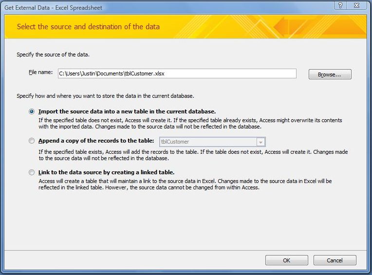
2. Click the BROWSE button on the first page of the wizard and select the text file which has been saved in your downloads folder. Leave the top radio button selected - it reads "import the source data into a new table in the current database". Click OK at the bottom of the wizard window.
3. The next page (see screenshot below) shows a sample of the data we are importing. At the top it reads "Your data seems to be in a delimited format. If it isn't, choose the format that more correctly describes your data". If you look at the sample of data displayed, you see each field is separated by a comma. We can therefore leave the "Delimited" radio button checked, and click NEXT.
4. The next page of the wizard (see screenshot below) asks us to choose the delimiter that separates our fields. As we noted above, our data is separated by commas, so we should now select the "Comma" radio button. We also need to click the "First Row Contains Field Names" tickbox. You may get pop up message explaining some of the field names have been modified to make them compatible with Access. This is fine. Just click OK. We can now click NEXT to move on to the next page of the wizard.

5. This page (see screenshot below) gives us the option to specify information about each of the fields we are importing. This includes specifying the data type for the field. We are going to change the data type for the price_paid field from SHORT TEXT to CURRENCY. To do this, highlight the price_paid column and select CURRENCY from the DATA TYPE combo box. We will also change the data type on the deed_date field from SHORT TEXT to DATE WITH TIME. Another thing we are going to change is the index type (ie the Indexed field option) on the unique_id field from "Yes (Duplicates OK)" to "Yes (No Duplicates). This will ensure the data set does not contain any duplicate records.
At this stage we can clean the data set further by excluding any fields that we do not need. To do this, highlight the field for exclusion and tick the "Do not import field" tick-box in the Field Options section. We are going exclude the estate_type field, and all the fields from transaction_category and after.
We can then click NEXT to continue.
6. The next page of the wizard lets us choose a primary key. There are three options: these are "Let Access add primary key", "Choose my own primary key" and "No primary key". We are going to select our own primary key, so tick the middle option and select the "unique_id" field from the combo box list. Then click NEXT.
7. In the last page of the wizard we are asked to choose a name for the table into which our data is to be imported. Entry the table name "tblSalfordHouseSales" and click FINISH.
We can now take an initial look at the table of data we have imported. Go to the Access navigation pane and open tblSalfordHouseSales (see screenshot below).
As we can see, the data set contains 2946 records. Each record provides information about the sale of a given property and consists of 13 fields. Some of most useful fields we shall be using for data analysis in this tutorial are price_paid, deed_date and postcode. We also have the option of analysing house sales by property_type and whether the property is a new_build.
Checking the Data
Now we have imported the data set into Access, we can start checking it's accuracy. However, before we start, lets make a copy of the imported table so we can undo any changes that we make without having to repeat the download and import process. Do this by right clicking tblSalfordHouseSales in the navigation pane and select COPY from the context menu. Then simply right click a blank space in the navigation pane and select PASTE. A window opens where we can enter a new name to call the table we are pasting, and select which paste option we would like. We are going to call the new table "tblSalfordHouseSalesOriginalData" and select the Structure and Data paste option. This will paste a new table based on the same structure, and containing the same data, as the one we copied. Then click OK.

The first thing we are going to check are the postcodes (zip codes) in our dataset. Since the data we have downloaded is for the Salford area of Greater Manchester, each record in the dataset should start with one of the following values in the postcode field: - M3, M5, M6, M7, M27, M28, M30, M38, M44, and M50 (after which there is a space followed by the second part of the postcode) . As such, we are going to create a query which groups the data into groups comprised of the first three values of the postcode, and provide some basic aggregate information for each grouping. From this information, we should be able to pick out any obvious anomalies contained in the data.
Create Query to Group & Aggregate Postcode Data
1. Create a new query by clicking the QUERY DESIGN icon on the CREATE ribbon.
2. Click the ADD TABLES icon (on the QUERY DESIGN ribbon) to display the ADD TABLES sidebar if it is not visible already.
3. Drag the tblSalfordHouseSales table from the tables list in the sidebar over to the QUERY DESIGN window.
4. Click the TOTALS icon in the SHOW/HIDE group of the QUERY DESIGN ribbon. This adds a TOTAL row to the QUERY DESIGN grid. This enables us to specify whether the field is to group the data contained therein, or perform an aggregation on it.
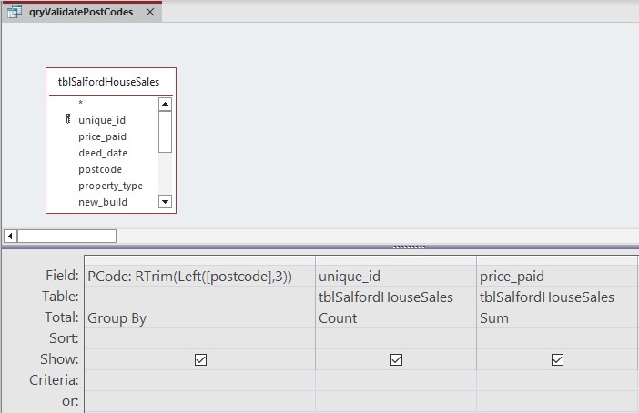
5. The first column in the query grid (see screenshot above) is going give us a list of postcode groups. All the post code groups in the Salford area (see above) are 2 or 3 characters long. So to extract the postcode group value from the value stored in the postcode field , we are going to create a calculated field in the first row of the first column of the query grid. The calculation is based on the postcode field in tblSalfordHouseSales and utilises the Left string function to take the first 3 characters of the field value. This is enclosed within a RTrim function to remove the right blank space if the postcode group is two characters rather than three. It is written as follows:
RTrim(Left([postcode], 3))
We will use the alias PCode as the field name. This is written ...
PCode:
... directly before the RTrim function syntax. So altogether the first row of the first column in the query grid (see screenshot above) will read ...
PCode: RTrim(Left([postcode], 3))
We then set this field to GROUP BY in the TOTALS row.
6. In the second column of the query grid, we are going to count the number of records within each postcode group. So, in the ADD TABLES side bar, drag the unique_id field from tblSalfordHouseSales down to the first row of the second column in the query grid, and select COUNT from the drop down list in the TOTALs row.
7. In the third column of the query grid we are going to SUM the total of price_paid to give us the total price paid within each postcode group. So drag price_paid from tblSalfordHouseSales down to the first row of the third column in the grid, and select SUM in the TOTALs row.
8. Click the RUN or DATASHEET icon in the RESULTS group of the QUERY DESIGN ribbon to see the query results.
Looking at the query results above, we can see that most of the properties have a post code in the Salford area - these are M3, M5, M6, M7, M27, M28, M30, M38, M44, and M50. However there are three properties which do not have any postcode, and one property which has a postcode starting with WA1. Taken together these come to a total value of £10,249,999. In order to ensure our data set is accurate, we need to investigate why these properties do not have a Salford post code and remove them if necessary. To do this we shall create another query to get the full information for the dubious records.
1. Repeat steps 1 to 3 above to create a new query based on the tblSalfordHouseSales table.
2. Drag the asterix * from the tblSalfordHouseSales table down to the first row of the first column on the query design grid. The asterix is a quick way to include all the fields in the table without having to drag each one individually. However, if we need to enter a criteria for a particular field (which we do) we can still drag that field down separately ..
3. As such, drag the postcode field down to the first row of the second column in the grid.
4 Click the CRITERIA row in the postcode column and enter the following expression:
Is Null or Like "WA1*"
 |
The criteria Is Null Or Like "wa1*" will pull out any record containing a
postcode with a null value or a value starting with "wa1". |
5. Click the RUN or DATASHEET view icon in the RESULTS group of the QUERY DESIGN ribon the see the query results
The first record returned by our query is for a property with the postcode WA14 5DY which (if you scroll across) is actually located in the town of Altrincham. If you are familiar with the geography of Greater Manchester you will know that this town is in the borough of Trafford rather than Salford. As such, this record does not belong in our dataset and should be removed. When we examine the data for the remaining three records, it is apparent that they pertain to land in a commerce park, a parking space, and a brown field site. As such they fall outside the scope of our interest in house sales, and can also be removed from our dataset. Its worth reflecting that had we not done this check, our dataset would have inaccurate to the value of £10,249,999.
A good way to remove these records from the dataset is to go back into QUERY DESIGN view and change the query type from SELECT to DELETE.
After changing the query type from SELECT to DELETE, you will see an addition row appear in the query grid entitled "Delete". You will also see that Access has filled in the values for this row. In the first column it has added "From" which means the records are being deleted from the tblSalfordHouseSales table, and in the second column it has added "Where" which means all records in the table matching our criterion Is Null Or Like "WA1*" will be deleted.
Click the RUN icon in the RESULTS group of the QUERY DESIGN ribbon to run the delete query.
Access will display a warning dialog saying that the 4 rows containing dubious records are going to be deleted from our table.
Click YES to continue the delete operation.
If we now go back and reopen tblSalfordHouseSales the record count will now show 2942 records, 4 less than the 2946 records we had previously.
There are many other checks that we can do to ensure our dataset is clean, but the steps mentioned above give us an idea of how we can use Access's queries and other features in this process. Let us now move on and see how we can use Access to analyse our dataset.
Analysing Data with Access Queries
To illustrate how Access can be used to make sense of our housing sale dataset, we are going to create a number of price bands and count the number of sales in each band. This will give us a basic understanding of the housing market in Salford during 2023.
This task will involve the creation of a subquery for each individual price band, and a parent query to pull together the sale counts within each band, showing them all in one row of aggregate data. Lets begin with the subqueries.
We are going to create a total of seven price bands as follows:
PRICE BAND SUBQUERY
< £100,000 qrySubBelow100K
>= £100,000 and < £200,000 qrySub100Kto200K
>= £200,000 and < £300,000 qrySub200Kto300K
>= £300,000 and < £400,000 qrySub300Kto400K
>= £400,000 and < £500,000 qrySub400Kto500K
>= £500,000 and < £1,000,000 qrySub500Kto1000K
>= £1,000,000 qrySubAbove1000K
Each of the above queries is based on the unique_id and price_paid fields of tblSalfordHouseSales. Once again, the query is going to use the TOTALS row in the QUERY DESIGN grid because we need to aggregate the data returned. We are going to set up our query to count the number of rows returned in the dataset when we add a criterion to the price_paid field. To do this we shall set the value in the TOTALS row of the unique_id column to COUNT, and the value of the TOTALS row of the price_paid column to WHERE. All we need to do then is enter the criterion in the CRITERIA row of the price_paid column. For example, when we create qrySubBelow100K to count the number of sales less than £100,000 the criterion we enter is <100000 as in the screenshot below:
 |
You may have noticed how the tickbox in the SHOW row
of the QUERY DESIGN grid is unticked when we select WHERE
in the TOTAL row for price_paid. This is because the only purpose
of the price_paid column is to filter the rows to be included in the
count of unique_id's. |
When we run the query a single row and column is returned with the count of
unique_id's matching the query criterion entered for
price_paid. For records with a price paid value less than £100,000 this should value should be
140.
Here are the instructions for creating the subqueries for the seven price bands. We will need to repeat this process seven times for each of the subquerie:
1. Create a new query by clicking the QUERY DESIGN icon on the CREATE ribbon.
2. Click the ADD TABLES icon (on the QUERY DESIGN ribbon) to display the ADD TABLES sidebar if it is not visible already.
3. Drag the tblSalfordHouseSales table from the tables list in the sidebar over to the QUERY DESIGN window.
4. Click the TOTALS icon in the SHOW/HIDE group of the QUERY DESIGN ribbon
5.In the first column of the QUERY DESIGN grid, select the unique_id field from the drop down list in the top row.
6. We now need to go down to the TOTAL row in the first column and select COUNT from the drop down list.
7. In the second column of the QUERY DESIGN grid, select the price_paid field from the drop down list.
8. Going down to the TOTAL row of the second column, select WHERE from the drop down list.
9. We now need to enter the criterion in the CRITERIA row of the second column. The criterion we enter depends which of the seven subqueries we are working on. The criterion for qrySubBelow100K, for example, is <100000. The criteria for all seven queries are listed in the table below.
10. Click the SAVE icon at the top left of the screen and the name of subquery that we were creating.
WHERE CRITERIA SUBQUERY
< 100000 qrySubBelow100K
>= 100000 AND < 200000 qrySub100Kto200K
>= 200000 AND < 300000 qrySub200Kto300K
>= 300000 AND < 400000 qrySub300Kto400K
>= 400000 AND < 500000 qrySub400Kto500K
>= 500000 AND < 100000 qrySub500Kto1000K
>= 1000000 qrySubAbove1000K
In addition to the seven subqueries above, we shall also create another subquery (qrySubCountAll) to give us a grand total for 2023 Salford house sales across all price bands. This subquery is the same as those we created above, except we do NOT need the price_paid column or any WHERE clause therein. We just need the COUNT in the unique_id column as in all the previous subqueries:
When this query is run we get the same output format as the previous seven subqueries (see screenshot below). The result is a count of all house sales in tblSalfordHouseSales. This should be 2942.
Now we have created all our subqueries we can begin work on the parent query which pulls all the subquery results together in one row of aggregate data.
The Parent Query
We are going to call our parent query qryHousePriceGroups. Each column in the query will display the aggregate total count of house sales for each of the price bands. The last column will display the grand total. To do this we will need to add all 8 subqueries we created to the QUERY DESIGN grid window and use the appropriate subquery as the data source for each of the parent query columns.
As we can see in the screenshot above, we have given each column name an alias such as "Below 100K" and "100K to 200K". This will make the query output easier for users to read and understand.
Here are the step by step instructions for creating the parent query.
1. Create a new query by clicking the QUERY DESIGN icon on the CREATE ribbon.
2. Click the ADD TABLES icon (on the QUERY DESIGN ribbon) to display the ADD TABLES sidebar if it is not visible already. Then select the QUERIES tab at the top of the sidebar. You should see all the subqueries that we have created previously.
3. Drag all 8 subqueries over to the QUERY DESIGN window. We will now start to dragging the CountOfUnique_id fields from each subquery onto the QUERY DESIGN grid below.
4. The first CountOfUnique_id field we are going to drag is from the qrySubBelow100K subquery. Drag this down to the cell in the top row of the first column in the grid.
5. We shall now enter the alias name for the column. We do this by typing the name Below 100K in the same cell just before CountOfUnique_id separated from it by a colon as follows:
Below 100K: CountOfUnique_id
6. In the top row of the next column, we are going to drag CountOfUnique_id from the qrySub100Kto200K subquery. We shall give this the alias 100K to 200K.
7. Repeat step 6 for each of the subqueries using the following alias's:
200K to 300K:
300K to 400K:
400K to 500K:
500K to 1000K:
Above 1000K:
All:
When we run the query we should get this result:
As we can see, out of a total of 2,942 house sales, the vast majority fall within the 100K to 200K, and 200k to 300K price groups. The 100K to 200K group contains 1,258 sales, and the 200K to 300K group contains 992 sales, giving a total of 2,250 sales out of 2,942, or 76% of the total 2023 Salford housing sale count. The figures also reflect the fact that Salford has some poorer districts as well as those which are very affluent. There were 140 house sales (5%) with property values of less than £140,000, but 100 sales (5%) with values between £500,000 and £1000,000, and 26 sales (1%) above £1000,000.
Lets end by showing this data visually in a clustered column chart embedded in an Access report. Here are the step by step instructions:
1. Click the REPORT DESIGN icon in the REPORTS group of the CREATE ribbon.
2. Resize the REPORT DESIGN grid so we get a larger section of screen in which to create the chart.
3. Click the INSERT MODERN CHART drop down menu in the CONTROLS group of the REPORT DESIGN ribbon. We are going to select the CLUSTERED COLUMN CHART from the COLUMN submenu.
4. The cursor will now change to a small chart symbol. Position the cursor in the top left hand corner of the DETAIL section of the design grid. A small chart will embed itself on the grid. At this stage we just have sample data displayed in the chart.
5. Resize the chart by clicking it's border on the bottom left corner and dragging the corner down and across so we get a bigger chart.
 |
| New chart showing sample data. |
6. We will now connect the chart to our parent query. We can do this from the CHART SETTINGS sidebar. Click anywhere inside the chart so it is selected. Then click the CHART SETTINGS icon in the TOOLS group of the REPORT DESIGN ribbon (if the sidebar is not displayed already).
7. Click the QUERIES radio button under DATA SOURCE, then select the parent query that we created earlier from the drop down list.
8. Go down to the VALUES (Y axis) section below. You will see a list of checkboxes with the price bands we created in our query. Tick each of the boxes except ALL. That is from Below 100K down to Above 1000K. You will notice there is a COUNT OF aggregate function contained within brackets after each of the check box labels. We need to change the aggregate function to NONE by clicking the drop down list which appears when you hover the mouse over the text. You should now see the data from our parent query appear on the chart. We now need to customise the appearance of the chart to make it more user friendly.
 |
Chart showing parent query data ready
to be customised. |
9. The first customisation we shall make is the addition of a data label above each chart column. This shows the value for the count of sales for each of the price bands. To do this select the FORMAT tab at the top of the CHART SETTINGS side bar. Select the first price band Below 100K from the drop down list under the DATA SERIES title. Then tick the Display Data Label checkbox.
You should now see the value 140 appear above the Below 100K column on the chart.
10. Select the next price band from the Data Series drop down list and tick the Display Data Label checkbox. Do this for the rest of the price band columns on the chart.
11. For the remaining customisations, we are going to use the chart property sheet. Click anywhere inside the chart so it is selected, then click the PROPERTY SHEET icon from the TOOLS group of the REPORT DESIGN ribbon.
12. The next customisation we are going to make is the addition of a chart title. Select the FORMAT tab on the property sheet and locate the HAS TITLE and CHART TITLE properties further down the sheet. Ensure the HAS TITLE property is set to YES, and enter "2023 Salford House Sales" for the CHART TITLE property value.
13. We shall next move the legend from the top of the chart to the bottom. To do this locate Legend Position also on the FORMAT tab of the property sheet. Change the property value to "bottom".
14. The final customisations we are going to make involve adding a title to the vertical axis and remove the text saying "140" below the horizonal axis. To do this locate the primary values axis title on the property sheet and change the value to "Count of Sales"; and then locate the category axis font color property, click the ellipse button (...) in the value cell, and select white from the colour chart. This will hide the unwanted text from view.
15. We can now open the report by clicking the REPORT VIEW button on the VIEWS group of the REPORT DESIGN ribbon. The result should look like the screenshot below:
We can now see the data from our parent query in visual form, thereby gaining a clearer view of the concentration of house sales in the 100K to 200K, and 200K to 300K price bands.
There are, of course, many other dimensions we can use to analyse our data. For example, we can create queries to group house sales according to property type, and find out the average value in each group. We could also have downloaded a larger dataset which includes sales over a number of years, and create a chart showing how prices have changes over particular timespans. I intend to cover areas such as these in future posts.